Lab 1
Materials for class on Friday, January 11, 2019
Contents
Things we’ll do
- Convert nominal values to real values
- Rescale the CPI to a different year
- Calculate inflation rate
- Calculate average inflation over time
- Compounding inflation
Inflation-related formulas
Nominal to real
Converting nominal values (the numbers written down at the time) to real values (the numbers in today’s / another year’s dollars):
\[ \text{Real value} = \frac{\text{Nominal value}}{\text{Price index / 100}} \]
Shifting CPI
Shifting the price index to a different year:
\[ \text{Price index}_{\text{new year}} = \frac{\text{Price index}_{\text{current year}}}{\text{Price index}_{\text{new year}}} \times 100 \]
Inflation rate
The inflation rate is the percent change in CPI between two periods. The formula for percent change is:
\[ \text{% change} = \frac{\text{New} - \text{Old}}{\text{Old}} \]
or
\[ \text{% change} = \frac{\text{Current} - \text{Previous}}{\text{Previous}} \]
Pay attention to the time periods in data from FRED.Or anywhere, really.
Datasets like GDP are reported quarterly, while the CPI is monthly. If you need to calculate the annual change (or annual inflation), make sure you either (1) use the same month or quarter as your current and previous times (i.e. January 2016 and January 2017), or (2) add all the percent changes within the year (i.e. add the rates from January 2016, April 2016, July 2017, and October 2017).
Compounding inflation
The compound average inflation rate is the percent that if the CPI had grown at that rate, compounded, from the start year to the end year, the same CPI would occur in the end year. To calculate this, use the formula for compounding interest, where \(A\) is the CPI or price at the end of time period we’re concerned about, \(P\) the CPI or price at the beginning of the time period we’re concerned about, \(n\) is the number of times the rate is compounded each year, \(t\) is the number of years, and \(r\) is the rate that you want to solve for:
\[ A = P (1 + \frac{r}{n})^{nt} \]
If we assume interest is compounded once a year, \(n\) is 1 and can disappear. This simplifies to:
\[ \text{CPI}_{\text{new}} = \text{CPI}_{\text{old}}(1 + r)^{t} \]
We can rearrange the formula so that \(r\) is on the righthand side by dividing, exponentiating, logging, and subtracting:
\[ r = exp(\frac{ln(\frac{\text{CPI}_{\text{new}}}{\text{CPI}_{\text{old}}})}{t}) - 1 \]
Alternatively, instead of assuming annually compounding interest, we can also assume exponential growth (or continually compounding interest), which uses the following formula (again where \(A\), \(P\), \(r\), and \(t\) are the prices in the last year, prices in the first year, the rate, and the number of years:
\[ A = Pe^{rt} \]
Or
\[ \text{CPI}_{\text{new}} = \text{CPI}_{\text{old}}e^{rt} \]
We can again rearrange the formula so that \(r\) is on the righthand side:
\[ r = \frac{ln(\frac{\text{CPI}_{\text{new}}}{\text{CPI}_{\text{old}}})}{t} \]
Inflation fun with Excel
Download these files:
I’ll put the complete version of the Excel file here after the lab.
Here’s the complete worked-out, cleaned-up example:
Inflation fun with R
Live code
Use this link to see the code that I’m actually typing:
I’ve saved the R script to Dropbox, and that link goes to a live version of that file. Refresh or re-open the link as needed to copy/paste code I type up on the screen.
Cleaner code
First, load the data (either from a file you downloaded and placed in an RStudio project, or directly from the class website):
library(tidyverse)  # Load ggplot, dplyr, tidyr, and friends
library(lubridate)  # Do cool stuff with dates
library(readxl)     # Read Excel files into R

# From your computer (make sure the path to fred_cpi.xlsx is correct)
fred_cpi_raw <- read_excel("fred_cpi.xlsx")
fred_gdp_raw <- read_excel("fred_gdp.xlsx")
If you use the mutate() function from dplyr, it’s easy to create new columns based on inflation adjustment math. You can also exctract CPI values for specific years using a combination of filter() and pull() and then shift the CPI around to a different year.
Here’s some income per capita adjustment:
cpi_2018 <- fred_cpi_raw %>%
  filter(year(Date) == 2018) %>%
  pull(CPI)

fred_cpi <- fred_cpi_raw %>%
  # Only look at a few columns
  select(Date, CPI, `Personal income`, Population) %>%
  mutate(income_per_capita = `Personal income` / Population) %>%
  mutate(real_income_per_capita = income_per_capita / (CPI / 100)) %>%
  mutate(cpi_2018 = CPI / cpi_2018 * 100) %>%
  mutate(real_income_2018 = income_per_capita / (cpi_2018 / 100))

# See what the first few values of each column are
glimpse(fred_cpi)
## Observations: 40
## Variables: 8
## $ Date <dttm> 1979-01-01, 1980-01-01, 1981-01-01, 1982…
## $ CPI <dbl> 68.5, 78.0, 87.2, 94.4, 97.9, 102.1, 105.…
## $ `Personal income` <dbl> 2005384000000, 2231943000000, 25088900000…
## $ Population <dbl> 225055000, 227225000, 229466000, 23166400…
## $ income_per_capita <dbl> 8910.640, 9822.612, 10933.602, 11774.976,…
## $ real_income_per_capita <dbl> 13008.23, 12593.09, 12538.53, 12473.49, 1…
## $ cpi_2018 <dbl> 27.48300, 31.29451, 34.98566, 37.87438, 3…
## $ real_income_2018 <dbl> 32422.37, 31387.65, 31251.67, 31089.55, 3…And here’s some GDP adjustment using the GDP deflator:
fred_gdp <- fred_gdp_raw %>%
mutate(gdp_per_capita = GDP / Population) %>%
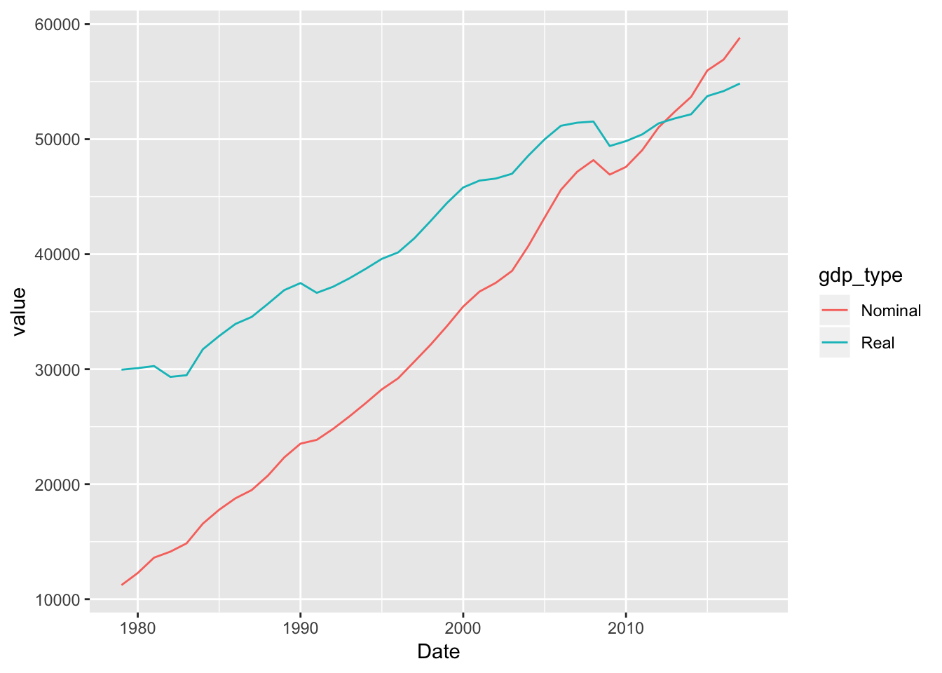
mutate(gdp_per_capita_2012 = gdp_per_capita / (`GDP deflator` / 100))Finally, here’s a demonstration of why it’s important to adjust for inflation. We can plot GDP per capita as both nominal dollars (what was written down at the time) and real dollars (2012 dollars):
# Make a dataset for plotting
plot_fred_gdp <- fred_gdp %>%
  # Only select the date and the GDP per capita variables + rename them
  select(Date, Nominal = gdp_per_capita, Real = gdp_per_capita_2012) %>%
  # Make this a long/tidy data frame, with one column for the GDP values and one
  # column for the type of value (real vs. nominal)
  gather(gdp_type, value, -Date)

# Plot this!
ggplot(plot_fred_gdp, aes(x = Date, y = value, color = gdp_type)) +
  geom_line()